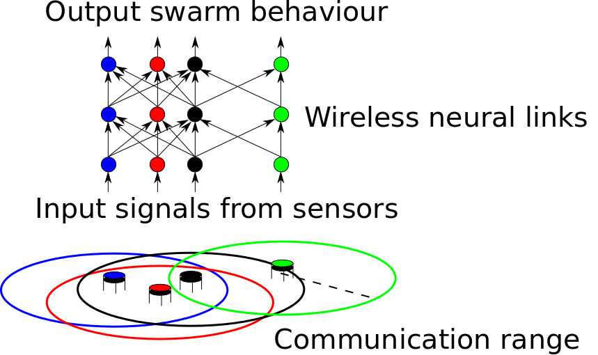
Collective Cognition & Sensing in Robotic Swarms via Emergent Group Minds

People: Michael Otte

The idea of a "group mind" has long been an element of science fiction. We use a similar idea across a robotic swarm to enable distributed sensing and decision making, and to facilitate human-swarm interaction.

All robots receive identical individual programming a priori and are dispersed into the environment. A distributed neural network emerges across the swarm at runtime as each robot maintains a slice of neurons and forms neural links with other robots within communication range. The resulting "artificial group mind" can be taught to differentiate between images, and trained to perform a prescribed (possibly heterogeneous) behavior in response to each image that it can recognize.

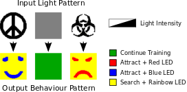
This animated video contains high level introduction to some of these ideas (it starts with a simpler idea to get started). See below for more videos of actual experiments.

In experiments we taught such a group mind to differentiate between three images: (1) peace sign, (2) biohazard sign, and (3) neutral gray pattern. The desired output behaviors the swarm learns to associate with each image are respectively: (1) form a blue smiley face, (2) form a red frowny face, or (3) keep training and display a yellow LED when finished.

In the first video (above) the swarm detects a peace sign and so creates a smiley face.

In the second video (above) the swarm detects a biohazard sign and so creates a frowny face.

A playlist of videos showing more experiments on swarms of 160-260 Kilobot robots can be found here.

It is important to understand that the group mind learns to differentiate between the patterns as a meta-entity. Many robots would be unable to differentiate between the smiley and frowny faces on their own. For example, any robot that receives the same input signal from both faces. In contrast, the swarm is able to leverage its distributed sensor network to detect patterns across the environment (similar to cells in a eye retina). The group mind neural network learns a mapping from different images to desired behaviors (which may vary spatially between robots for the same image).

Movement breaks the neural links and causes the group mind to dissolve. However, each robot retains the knowledge of which pattern was sensed, and which output behavior it should perform. The faces are physically created as robots that are not yet part of the face randomly move until they either join the face or leave the environment. It is assumed that robots have a library of such possible low level behaviors (e.g., randomly walk until some condition is met) but the mapping from possible images to output behaviors is learned at run-time.

The best place for more information is the IJRR 2018 journal paper , which includes many experiments, proofs of convergence , and a detailed algorithmic description. The earlier ISER 2016 conference paper is much shorter, with a limited focus on selected experiments.

top

RRT-X: Real-Time Motion Replanning in Dynamic Environments (with unpredictable obstacles)

People: Michael Otte, and Emilio Frazzoli

RRT-X is a motion replanning algorithm that allows a robot to plan, and then refine its motion during movement, while replanning (i.e., in its state space) if and when obstacles change location, appear, and/or disappear.

See the WAFR paper and/or the journal version for more information.

A playlist of videos showing the RRT-X motion planning/replanning algorithm in various spaces can be found here. The following are two videos from that list:

In the first (above), a holonomic robot is moving among unpredictable obstacles. The robot assumes that the robots will continue straight along their current trajectories---whenever this assumption turns out to be false, then the robot replans. The video show the real-time reaction of the robot. Colored lines represent the estimated paths of the robot/obstacles into the future. For visualization purposes nodes have been projected into the spatial dimensions of the state space.

In the second, a Dubins robot is provided with an inaccurate map of the world and must replan whenever its sensors detect that a new obstacle has appeared or an old obstacle has disappeared. The video show the real-time reaction of the robot. Color represents the distance to the goal, the search tree edges are drawn as straight lines between the nodes (not as the Dubins trajectories the robot will actually follow). For visualization purposes nodes have been projected into the spatial dimensions of the state space.

top

Efficient Collision Checking in Motion Planning

People: Joshua Bialkowski, Sertac Karaman, Michael Otte, and Emilio Frazzoli

Collision checking has been considered one of the main computational bottlenecks in motion planning algorithms; yet, collision checking has also been predominantly (if not entirely) employed as a black-box subroutine by those same motion planning algorithms. We discovered that a more intelligent, yet simple, collision checking procedure that essentially eliminates this bottleneck. Specifically (in math jargon), the amortized computational complexity of collision checking approaches zero in the limit as the number of nodes in the graph approaches infinity.

1

2

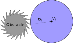
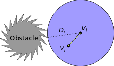
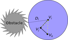
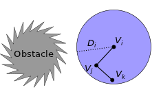
1) Instead of just returning a Boolean (true/false) value that represents "in collision" vs. "not in collision," our collision checking procedure returns the minimum distance to the closest obstacle. This obstacle-distance data (D i) is stored with the node (Vi) for which it was calculated (dotted black line), and represents a safe-ball (blue) around Vi (in non-Euclidean space the shape may not be a ball, but if the shape is convex then our method will still work).

2) When a new node (Vj) tries to connect to Vi with a new edge (black line) it can skip collision checking whenever Vj is closer than Di to Vi (in other words, if the new node is inside the safe-ball of the old node). Vj then remembers a pointer (dotted yellow) to Vi.

3

4

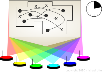
3) If a third node (Vk) wants to connect with Vj then collision checking can again be skipped if Vk is closer than Di to Vi (thanks to the convexity of the safe-ball around Vi). Vk then also remembers a pointer to Vi in case new nodes wish to attach to it (dotted yellow).

4) The same basic strategy also works if Di is an under-estimate of the distance from Vi to the nearest obstacle.

Click here to see the WAFR paper, which includes experiments and proofs. Or click here for the final IJRR journal version, which includes a more thorough treatment and includes extensions.

top

C-FOREST: Parallel Shortest-Path Planning with Super Linear Speedup

People: Michael Otte and Nikolaus Correll

Increasing the speed of path planning algorithms will enable robots to perform more complex tasks, while also increasing the speed and efficiently of robotic systems. Harnessing the power of parallel computation is one way that this can be achieved.

C-FOREST (Coupled Forests of Random Engrafting Search Trees) is an algorithmic framework for parallelizing sampling-based shortest-path planning algorithms.

C-FOREST works as follows:

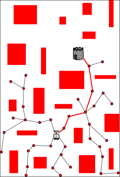
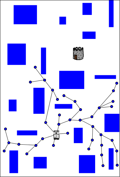
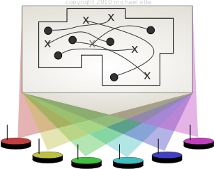
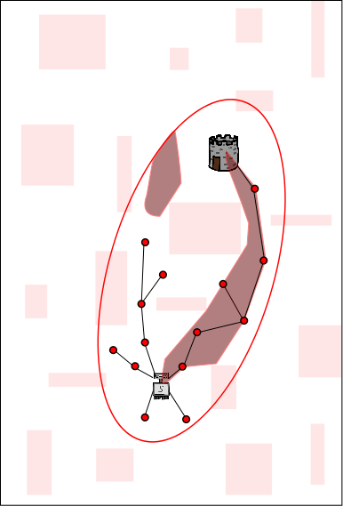
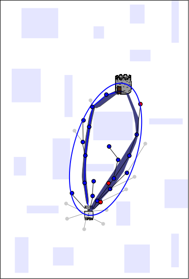
Each of the above three images represents the planning process that is happening on one of three different CPUs (red, blue, yellow). The problem being solved is for a robot (light gray, located in the lower-center of each image) to get to the tower (dark gray and brown above and to the right of the robot). Each CPU performs independent random planning until a better solution is found (this happens on the red CPU and the path is also red), and then the new (red) solution is exchanged between CPUs (as explained in the following images).

 

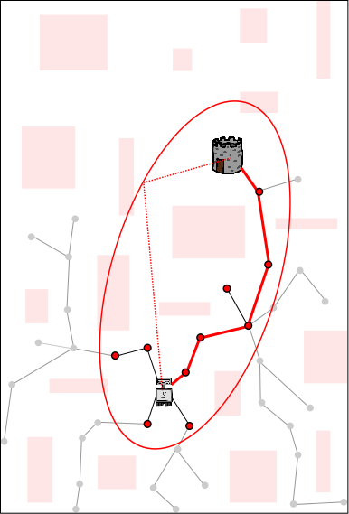
The length of this solution defines a boundary (here is is shown as red ellipse, as it would be if the robot were planning in 2D Euclidean space). Future samples are drawn from inside the ellipse (because those outside cannot yield better solutions). This increases the probability that an even better solution is found each time new random sample is chosen, and thus speeds up future planning. Existing nodes/branches can also be pruned (pruned nodes/branches are shown in gray), which decreases the time that it takes to connect future nodes to the tree (each time a new node is connected to the tree, we must find the best old node to connect the new node to; this search takes longer when there are more nodes, even though we use advanced data structures such as KD-trees). Sharing the length of the solution (from red CPU to blue and yellow CPUs) gives the advantages of knowing the red path to the other CPUs.

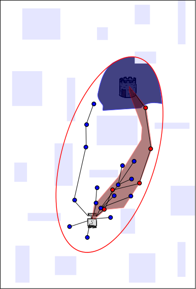
The dark shaded regions represent areas in the search space from which new samples will yield better paths. Note that those depicted here are only a cartoon approximation; in practice it is usually impossible to calculate this sub-space explicitly---which is why we use random sampling to begin with. Sharing the path itself increases the size of the sub-space from which new samples will yield better paths on the other CPUs. In this example, sharing the path from the red CPU to the blue and yellow CPUs further increases the probability of finding an even better solution on the blue and yellow CPUs.

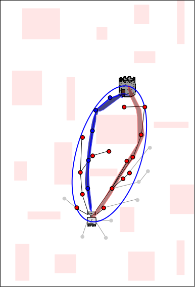
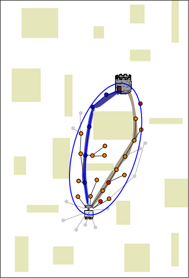
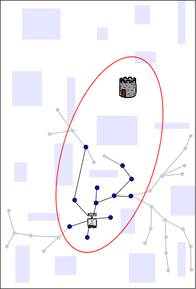
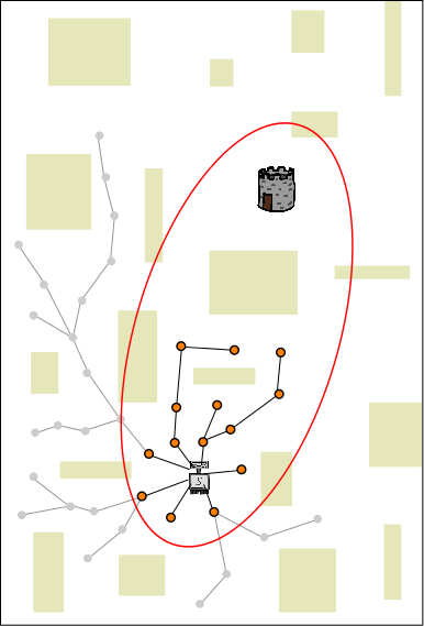
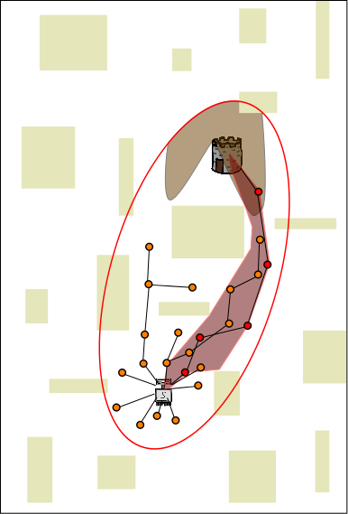
As more solutions are found (blue in this example), sharing the data among CPUs ensures that all CPUs can always prune, sample and improve their solutions based on the best solution known to any CPU.

Here are some of our results comparing C-FOREST to OR-parallelization (both use the RRT* planning algorithm) on a manipulator-arm path planning problem. Note that results are shown in terms of Speedup and Efficiency.

Speedup: (S) How many times faster an algorithm runs on a parallel architecture with N CPUs than it does on an architecture with 1 CPU. Efficiency: (E) is calculated as E = S/N and measures the relative power use of solving the same problem on an N CPU architecture vs. a 1 CPU architecture.

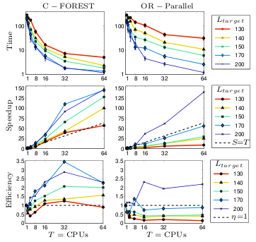
Not only does C-FOREST perform better than OR-parallelization on nearly all trials, C-FOREST also has super-linear speedup on nearly all trials!

super-linear speedup: speedup such that S > N (or E > 1).

C-FOREST can theoretically be used with any sample-based shortest-path planning algorithm such that, if it were allowed to use an infinite number of samples, then it would find the optimal solution with probability 1. (In formal math jargon: any algorithm that almost surely finds the optimal solution, in the limit as the number of samples approaches infinity).

See the paper and/or my PhD thesis for more experiments, as well as a full description of C-FOREST.

Here is a link to C-FOREST Code.

top

Any-Com Multi-Robot Path Planning

People: Michael Otte and Nikolaus Correll

Multi-robot path planning algorithms find coordinated paths for all robots operating in a shared environment. 'Centralized' algorithms have the best guarantees on completeness, but they are also the most expensive. Centralized solutions have traditionally been calculated on a single computer.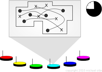

     
Solutions via a single robot (left) and an ad-hoc distributed computer (right).

In contrast, I combine all robots into a distributed computer using an ad-hoc wireless network. Since the network is wireless, the distributed planning algorithm must cope with communication disruption. The term 'Any-Com' implies graceful performance declines vs. increasing packet loss.

My Any-Com path planning algorithm works as follows:

• Each robot performs independent search in the combined configuration space of the entire team using a random tree algorithm.
• Better solutions are broadcast throughout the team whenever they are found.
• Robots that receive better solutions can use them to prune their own search trees, and also to avoid building new branches in places that cannot possibly lead to even better solutions.

Here is the paper:

Michael Otte and Nikolaus Correll.
Any-Com Multi-Robot Path-Planning: Maximizing Collaboration For Variable Bandwidth. In The 10th International Symposium on Distributed Autonomous Robotic Systems (DARS), Lausanne, Switzerland, November 2010.

More recently I have been using multiple ad-hoc distributed computers in a single environment. Each robot starts in its own team, and teams are combined if their solutions conflict. This helps reduce the complexity of the problem per distributed computer.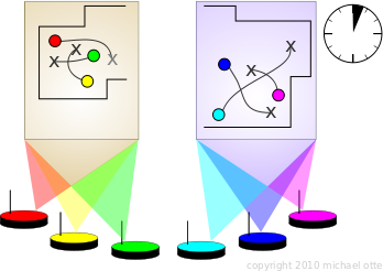

Two non-conflicting ad-hoc distributed computers.

This is discussed in the following paper:

Michael Otte and Nikolaus Correll. Any-Com Multi-Robot Path-Planning with Dynamic Teams: Multi-Robot Coordination under Communication Constraints. In International Symposium on Experimental Robotics (ISER), New Delhi, India, December 2010.

In early work on the Any-Com idea, I also experimented with task allocation:

Michael Otte and Nikolaus Correll. The Any-Com Approach to Multi-Robot Coordination. In IEEE International Conference on Robotics and Automation (ICRA), Workshop on Network Science and Systems Issues in Multi-Robot Autonomy (NETSS), Anchorage, USA, 2010. Poster.

Finally, the most recent version of all of this work (and more!) is in my PhD Thesis.

top

2D Robotic Path Planning (Extracting Paths from Field D*)

People: Michael Otte and Greg Grudic

Path planning algorithms attempt to find a path from the robot's current location to a goal position, given information about the world. World information is usually stored in a map, but it can be organized in many different ways. A common idea is to break the world into grids, and then have each grid remember a piece of information about a specific part of the world: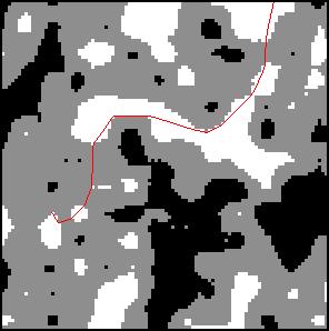

light-dark represents terrain that is easy-hard to navigate, red is the resulting path.

Or something a little more obvious...

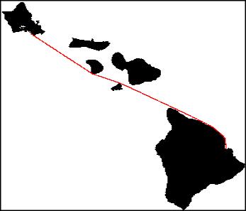
white/black are water/land, red is a sea route from Hilo Bay to Waikiki (Hawaii)

In 2009 I found a better way to extract paths from this type of map. Here is a simple example (blue is my method, red is the previous method):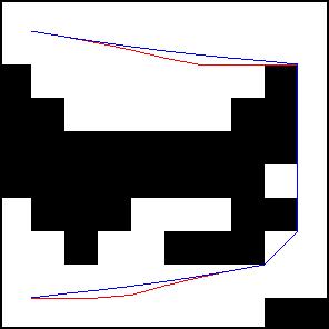

white/black are free/obstacle.

Here is the paper:

Michael Otte and Gregory Grudic. Extracting paths from fields built with linear interpolation IEEE/RSJ International Conference on Intelligent Robots and Systems. St. Louis, United States, 2009.

and here is the code.

My idea is built on a modified version of the Field D* Algorithm [1], so it is equipped to update the cost-to-goal field with a minimum amount of effort if/when world information changes.

top

Path Planning in Image Space (DARPA LAGR)

People: Michael Otte, Scott Richardson, Jane Mulligan, Greg Grudic

I began working with mobile robotics while involved with the Defense Advanced Research Project Agency (DARPA) Learning Applied to Ground Robotics (LAGR) program. Here is a picture of the LAGR robotic platform: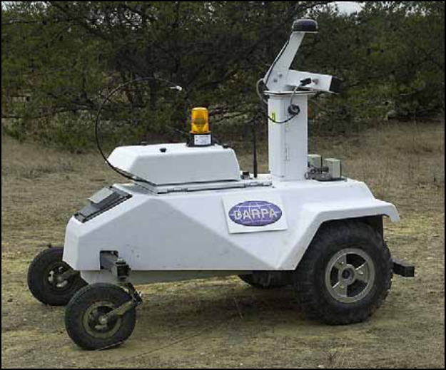

(Note that I borrowed this image from a slide presentation given by former LAGR P.I. Dr. Larry Jackel)

The robot's task was to navigate to a predefined coordinate (as fast as possible given a 1.3 m/s speed cap).  The basic idea of LAGR was that the robot should be able to learn about the environment as it interacts with it, thus improving the ability to navigate through the environment as time progresses. The robot's primary sensors include four digital cameras that are arranged in two stereo pairs. The stereo camera pairs provide scene depth information (similar to the way that human eyes do) and also color information. The range of the depth information is accurate to a maximum of 5 meters, but color information is only limited by the robot's line-of-sight.

One of the primary goals was to learn what colors were likely to be associated with the ground or obstacles, given a particular environment. This relationship can be learned in the near field, within the range of accurate depth information from the stereo cameras. Once learned, the ground vs. obstacle information can be extrapolated to the far-field as a function of color. This is important because it significantly increases the usable range of the sensor, giving the robot more information about the environment, and enabling it to make better decisions about what to do.

My part in this project was to create and maintain the mapping/path-planning system---the piece of software charged with remembering information that the robot has discovered about world traversability, and then calculating the "best" way to reach the goal given the robot's current position.

Here is a map that has been created from environmental traversability information: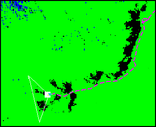

In the map, green-black represents ground-obstacle, dark blue means "unknown," the purple dashed line is the path that the robot has taken to get to its current location, the white triangle represents the robots field-of-view, the light blue rectangle is the robot, and the big white square is the goal. This is a happy robot because it has reached the goal.

Most path planners either operate in a Cartesian based top-down map like the one shown above, or a 3D representation of the environment. This means that camera information must be transformed into another coordinate space before it can be used. I developed methods that allow paths to be found directly in the coordinate space of raw camera information. This is like steering a car by looking out of the front windshield, instead of by looking at the car's position on a road-map.

Here is a picture showing ground vs. obstacle information (right) that is extracted from a stereo disparity image (center)---disparity is inversely related to depth. The RGB image is also shown (left).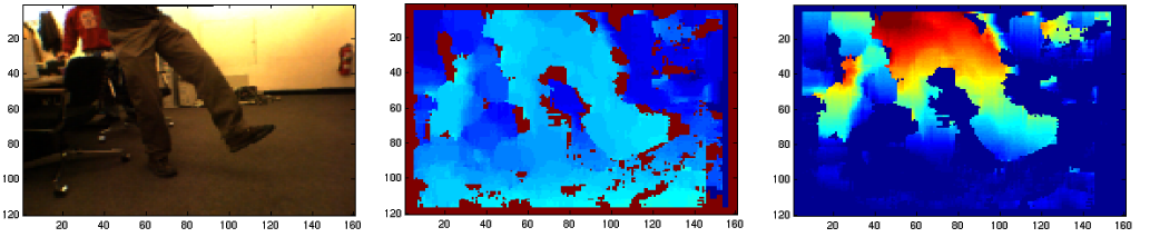

As demonstrated by a simple bale obstacle, paths can be found directly in this cost information (right):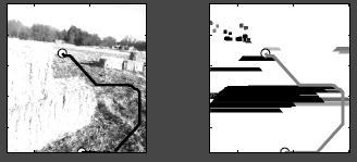

Note that the width of obstacles have been increased by 1/2 the width of the robot so that it will not collide with the obstacles if it follows the path.

Here is the paper I wrote about this idea (my Master's Thesis was an earlier iteration of this work):

Michael W. Otte, Scott G. Richardson, Jane Mulligan, Gregory Grudic. Path planning in image space for the autonomous robot navigation in unstructured outdoor environments. Journal of Field Robotics, Volume 26, Issue 2, February, 2009, p. 212-240. preprint version.

I found that using a version of this planner that simulates a 360 degree field-of-view in memory can provide a good local planner--that is, a system that is used to quickly find paths around immediate obstacles. However, the image planner cannot remember information about locations that have moved far away from the robot, thus it does not make a robust global planner--that is, a system that finds long-range paths.

top

Machine Learning Applied to Systems Data

People: Scott Richadson, Michael Otte, and Mike Mozer

Modern computer programs are very complicated, often hard to analyze, and may interact with lower levels of code in unexpected ways. Often programmers cannot predict how a piece of code will affect the given computer architecture that it runs on until it is actually executed (i.e. with respect to memory usage or runtime). Also, different architectures may respond differently to the same piece of code.

It has been shown that computer architectures exhibits phase behavior. That is, if a record of the architecture's operation sequence (i.e. execution trace) is sliced into many pieces, than many of these pieces can be divided into groups defined by similar behavior. For instance, here is a plot of the cycles per instruction (CPI) of a simple benchmarking program (gzip,ref2):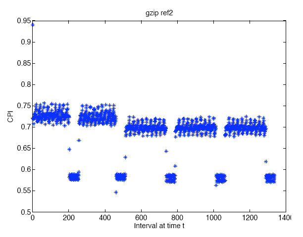

Thanks to Scott Richardson for making this figure.

As you can see, there appear to be two or three distinct phases of behavior, as well as a few intervals that are unique.

CPI is just one of many metrics that are used to evaluate an architecture's performance. When a new architecture is designed, it must either be fabricated or simulated in software. The former is expensive, while the latter is time intensive. For hardware dependent metrics such as CPI, architecture simulation may taking months of computation time (even to run a trivial program).

In order to speed up development, designers often choose to simulate only a fraction of the entire program. To date, simple machine learning tools have been used to cluster program intervals based on easily obtained software metrics, such as non-branching pieces of code (i.e. basic blocks). Once the clustering of a program execution trace is found, only one interval per cluster must be executed on the software simulated architecture to determine how the architecture will likely perform over the entire program.

In previous research we investigated whether or not more sophisticated machine learning techniques could provide advantages over the relatively simple methods that are currently used.

top

References:

• D. Ferguson and A. Stentz. Using interpolation to improve path planning: The field D* algorithm, Journal of Field Robotics, vol. 23, p.79-101, 2006

top